Trend and variability of NDVI of the main vegetation types in the Cape Region of Baja California Sur

Tendencia y variabilidad del NDVI de los principales tipos de vegetación en la región del cabo de Baja California Sur

Monitoring ecological processes is essential to understand their functions, changes and drivers; this knowledge is necessary to protect the natural environment and preserve biodiversity (Willis, 2015). Natural as well as anthropogenic mechanisms can cause fragmentation and degradation of natural forest in natural protected areas (NPAs) as well as outside NPAs either shrinks wildlife habitat or break the continuity of genetic exchanges amongst spatially isolated populations, and thus causes significant biodiversity loss (Franklin et al., 2002; Mallegowda et al., 2015). Vegetation is the main component of terrestrial ecosystems on earth and plays an important role in the water energy exchange, and biogeochemical cycles on terrestrial surfaces (Peng et al., 2012). The status of the vegetation is commonly used in assessments of productivity of natural and agricultural lands and declining, or browning, trend is considered to indicate land degradation (De Jong et al., 2011).

Vegetation is characterised by inter-annual and seasonal variations; variations in the surface vegetation coverage affect the balance of the regional ecosystems, studies on the variation in vegetation coverage basis of the protection of the ecological environment (Jiang et al., 2015). Over the past 3 decades, researchers developed methods for analysing time series and detecting trends with a view to detecting changes and even separate different type of changes (Eckert et al., 2015).

Remote sensing change detection methods improve conservation abilities by monitoring changes in ecological status and can assess management effectiveness without further disturbing the landscape, which are cost-effective techniques for measuring landscape-level temporal changes over a continuous area in combination with Geographic Information Systems (GIS) (Gillespie et al., 2018; Willis, 2015). A wide range of remote sensing data sources (e.g., hyperspatial, hyperspectral and active), such as Landsat is very good at mapping the dynamics of forest ecosystems in isolated regions and activities such as logging can be monitored in and around protected area boundaries (Gillespie et al., 2014; Nagendra et al., 2013), and products (e.g., vegetation indices) are available, such as the Normalised Difference Vegetation Index (NDVI) and Foliage Projected Cover (FPC) (Nagendra et al., 2013). The combination of both techniques is commonly used for ecological monitoring in a variety of research projects and programs although their utilization by protected area managers continues to be limited (Nagendra et al., 2013).

The NDVI has many merits, such as the simplicity of its algorithm and ability to roughly differentiate vegetated areas from other land cover types; it is also more effective at identifying green vegetation than other methods that rely on a single band; this algorithm is normalised transformation of the near infrared (NIR) to red (RED) reflectance ratio (ρNIR/ρRED), designed to standardise vegetation index value, so they are between -1 and +1 with 0 standing for “no vegetation” and negative values for “non-vegetated surfaces”, such as water or snow (Pang et al., 2017).One of the most important requirements to effectively use the NDVI is the scale, both spatial and temporal. Willis (2015) explained the importance of choosing the appropriate spatial and temporal resolution. For example, a high resolution (30 m pixel) sensor, such as Landsat, may be used to monitor vegetation community-type changes, but it is not appropriate to monitor species-type changes. The next scale factor that should be considered is temporal resolution; for how long should the process be measured and how often? Effective change detection should be performed over a time period of at least 10 years (Huang et al., 2009).

This study used NDVI data for the spatial and temporal vegetation analyses during the growing season (September- November) for the different vegetation community-types in the Cape Region (CR) from 2001 to 2015, differentiating the most important natural protected area, Sierra La Laguna Biosphere Reserve, from the rest of the region. The results suggested that a vegetation index with high spatial resolution (30 m) derived from Landsat 7 imagery could be used to describe spatial and temporal variability of vegetation cover by type in the study area. This method can be used to define specific conservation and management programs in this natural protected area to preserve local biodiversity in this emblematic Biosphere Reserve.

Materials and methods

The Cape Region lies at the southern tip of the arid peninsula of Baja California, Mexico (24º N, 110º W) (León-de la Luz et al., 2000; Fig. 1). The climate, according to Köppen’s classification ranges from hot and dry to very hot and very dry and has an annual mean temperature from 22°C to 24°C, which varies from 22.7°C on the western slopes to 23.5°C on the eastern slopes(García, 1973; León-de la Luz et al., 2000). The rainy season is concentrated from July to January with an average precipitation of 200 mm (León-de la Luz et al., 2000). In the lowlands, the climate is typically hot and dry while it is typically temperate and humid in the highlands. Annual rainfall changes with the slope aspect from 506 mm on the western side to 303 mm on the eastern side in the high hills. (Arriaga & Ortega-Rubio, 1988; Conanp, 2003; León-de la Luz & Breceda, 2006). Five main cities are located in the Cape Region: La Paz, San Juan de los Planes, Todos Santos, San José del Cabo, and Cabo San Lucas, and several towns surrounding the area (Fig. 1). In this region the pristine and isolated Sierra La Laguna is located; the biophysical characteristics of this mountain area justified the creation of the Sierra La Laguna Biosphere Reserve (SLLBR; Fig. 1); its delimitation is included between the parallels 23°42’ and 23°20’N and the meridians 109°46’ and 110°11’W (Conanp, 2003) in the municipalities of La Paz and Los Cabos in the extreme southern part of the state in the Cape Region where the highest elevation reaches 2,100 m asl.

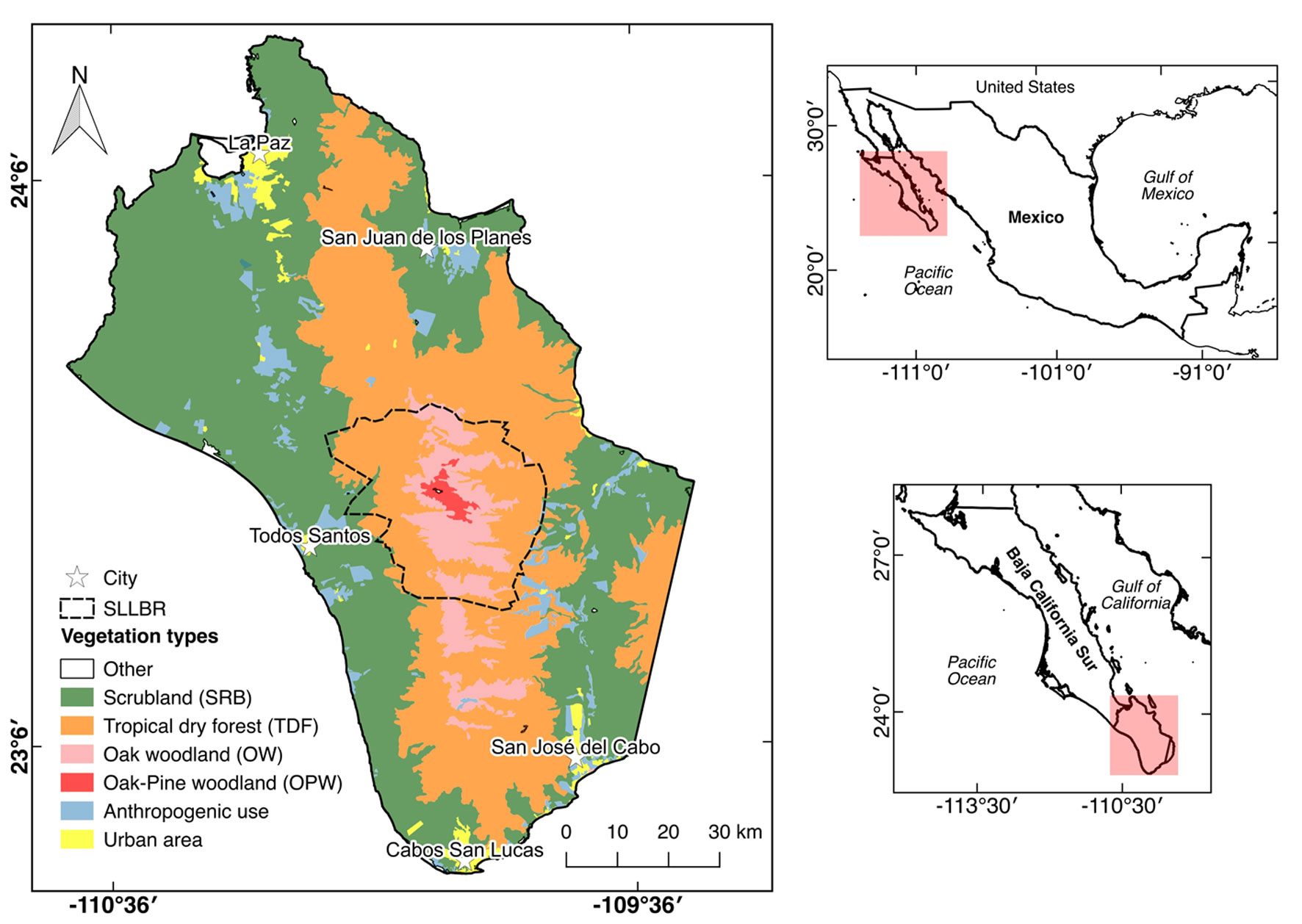
The Cape plant communities seem to be separated in their floristic composition and structural characteristics by their position along environmental gradients where elevation, rainfall levels and landform seem to be the most critical selective factors for plant life (León-de la Luz et al., 2000). The physical environmental factors favour the development of different vegetation types along an altitudinal gradient and are characterised by scrubland, tropical dry forest, oak woodland and oak-pine woodland (Arriaga & Ortega-Rubio, 1988).

The Sierra La Laguna can be considered as an ecological vegetation island in the middle of an arid environment where the unique tropical dry forest of the peninsula is found, and an oak-pine woodland is located in the highlands (Breceda et al., 2014; Padilla et al., 1988). From a floristic point of view, the reserve has been well studied, registering more than 900 species of vascular plants, of which approximately 89 are endemic (Rascón-Ayala et al., 2018).

Scrubland (SRB) is located from 0 to 500 m asl and comprises sarcocaule, sarcocrasicaule scrub and mezquital. The climate type, according to Köppen’s classification is very hot and very dry (García, 1973; León-de la Luz et al., 2000). The representative species of this vegetation type are Pachycereus pringlei Britton & Rose, Stenocereus gummosus (Engelm.) A.C. Gibson & K.E. Horak, Stenocereus thurberi (Engelm.) Buxb and Euphorbia eriantha Benth (Conanp, 2003).

The tropical dry forest (TDF) occupies an altitudinal zone from 500 to 1,000 m with hot and dry climate (García, 1973; León-de la Luz et al., 2000). The species that characterise this vegetation type are Lysiloma divaricatum J.F. Macbr, Jatropha cinerea Müll. Arg, Hesperalbizia occidentalis (Brandegee) Barneby & J.W. Grimes and Lysiloma candida Brandegee (Conanp, 2003).

Oak woodland (OW) is a transitional community between the TDF and OPW (800-1,200 m asl). Quercus tuberculata Liebm., Q. albocincta Trel., Dodonaea viscosa Jacq. and Heteropogon contortus Beauv. ex Roem. & Schult. are distinguished species in this vegetation type (Conanp, 2003).

The oak-pine woodland (OPW), located from 1,000-2,100 m asl, is dominated by species as Q. devia Goldman, Q. tuberculata Liebm, Pinus cembroides subsp. lagunae (Passini) D.K. Bailey, Arbutus xalapensis Kunth and Nolina beldingii Brandegee; its climate is classified as temperate humid (Arriaga & Mercado, 2004).

The study area was covered by 2 Landsat 7 scenes (path 34 and row 43; path 34 and 44). Landsat 7 satellite has imaged the Earth every 16 days from 1999 to date and carried the Enhance Thematic Mapper Plus (ETM+) sensor. Data was downloaded from the US Geological Survey server (USGS, https://www.usgs.gov) using EarthExplorer platform (https://earthexplorer.usgs.gov); an image of this compound sensor has 8 spectral bands that can be combined to different colour composition or processing; this study used images with less than 10% of cloud-cover from 2001 to 2015 for the growing season (September-November). This period (2001-2015) was used because images of the year 2000 had more than 10% of cloud-cover. Furthermore, only images for the growing season were used to describe vegetation variability when the CR exhibited the highest photosynthetic activity in the canopy, thus reducing variability of vegetation caused by seasonality.

The pre-processing data consisted of: 1) filling the gaps of Landsat 7 data of Scan Line Corrector (SLC), using raster (Hijmans, 2018) and rgdal (Bivand, 2018) libraries of R programming software (R Core Team, 2018); 2) performing radiometric calibration, atmospheric correction by the method of Dark Object Substract 1 (DOS1), which is based on image properties besides being the most widely used algorithm; for the detection of land-use changes (Prieto-Amparan et al., 2018), the Semi-Automatic Classification Plugin (Congedo, 2016) for QGIS 2.18 (QGIS Development Team, 2018) was used; 3) removing clouds and shadows through on-screen digitising was performed using the Cloud Masking Plugin (Corredor, 2018) for QGIS 2.18 (QGIS Development Team, 2018); 4) clipping and merging scenes for the study area polygon were performed using raster and rgdal libraries of R programming software (Bivand, 2018; Hijmans, 2018; R Core Team, 2018).

The NDVI values were derived by Landsat 7 images using spectral bands 3 (red) and 4 (near infrared, NIR), defined (Rouse et al., 1974) by:

NDVI = NIR-R / NIR+R    (1)

where NIR is the near infrared band and R is the red band.

Next, the NDVI data was pre-processed using maximum-value composites (MVCs) to generate annual values of the NDVI, which is formulated by:

NDVI_i = max (NDVI_i1, NDVI_i2, NDVI_i3,…, NDVI_ix)   (2)

where NDVI_i is the NDVI value of the ith year, and NDVI_i1 and NDVI_i2 are the NDVI values of the first and second halve date, respectively.

The NDVI mean, standard deviation, minimum and maximum values for each vegetation community-type, study area, biosphere reserve polygon, buffer zone polygon and study period (2001-2015) for the growing season (September-November) were computed.

Coefficient of variation (CV) is commonly used in vegetation research mainly to reflect the discrete degree of the NDVI data and the inter-annual/annual vegetation volatility (Jiang et al., 2015; Milich & Weiss, 2010; Tucker et al., 2001), which is calculated by:

CV_NDVI = σ_NDVI / NDVI    (3)

where, CV_NDVI refers to the NDVI coefficient of variation of each pixel for the period 2001-2015; σ_NDVI represents the standard variation of the NDVI value; NDVI is the mean NDVI value. Because the CV values vary depending on the region, CV was categorised in 5 classes (lower, low, moderate, high, and higher) using percentiles 0-20, 20-40, 40-60, 60-80, and 80-100%, which allowed comparing local vegetation variability more adequately.

This study described NDVI trends using the slope obtained from simple linear regression, using NDVI as a response variable and time (years) as predictor variable; two-tailed p-values were used to test the significance of these trends.

The spatial distribution of vegetation by type was obtained from the digitised map theme Land use and Vegetation at a scale of 1:250,000 Series VI, version 3 (INEGI, 2016). This map was clipped to the study area and merged similar land cover types into one category (Fig.1).

Four main vegetation community-types were obtained: scrubland (SRB) representing 50.69% of the study area and 3.32% for SLLBR area; tropical dry forest (TDF) 36.47% of the study area and 60.48% of SLLBR area; oak woodland (OW) 5.3% of the study area and 31.93% of SLLBR area; and oak-pine woodland (OPW) 0.45% of the study area and 3.96% for SLLBR area. Other areas were obtained as anthropogenic use (4.49%), urban area (2.11%), and another one catalogued as “other” representing mangroves and dunes, which is located out of the SLLBR area.

Results

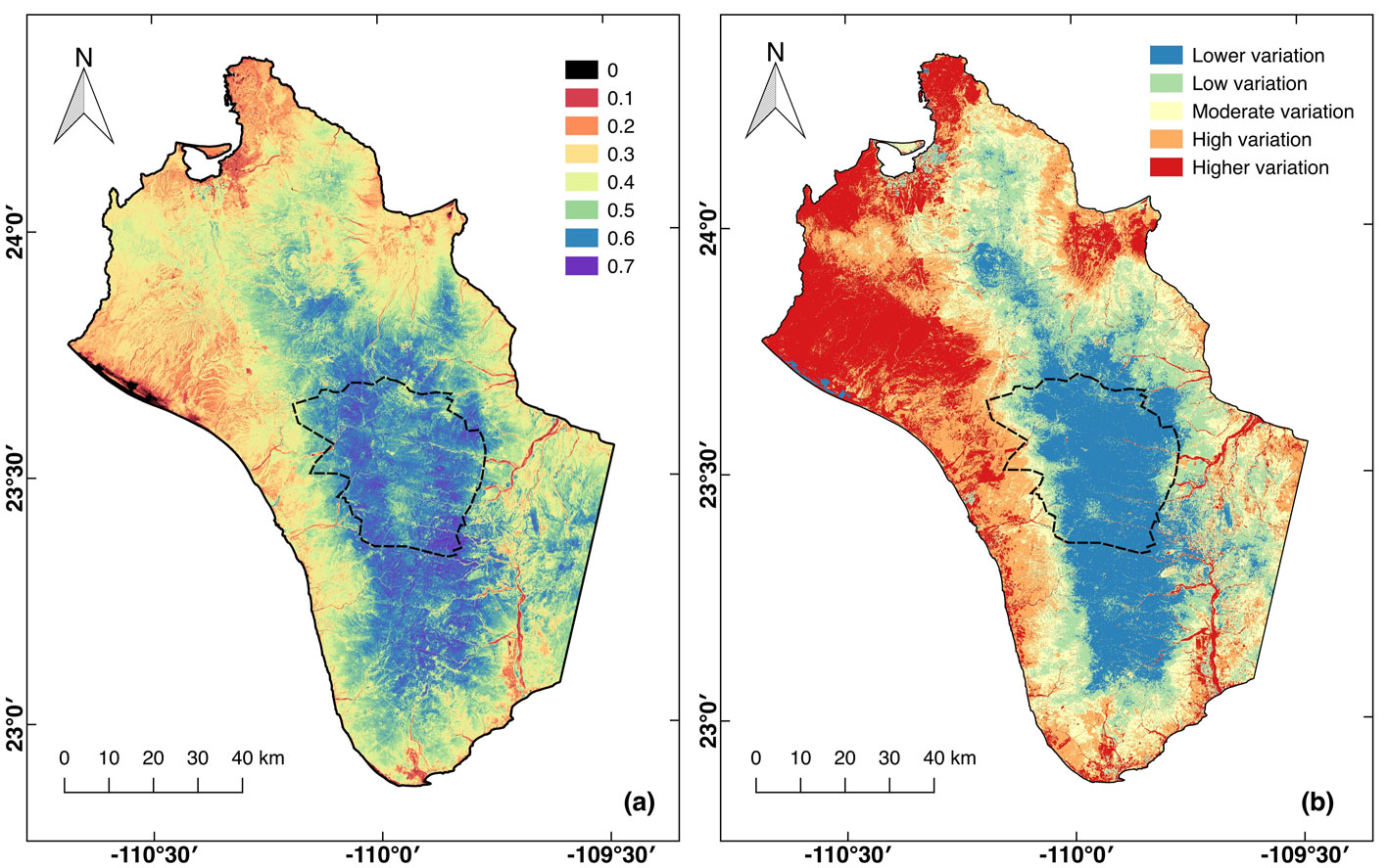
The spatial distribution of average NDVI for the growing season from 2001 to 2015 is shown in Fig. 2a where it gradually increased from the coast to highlands. The transition zone between TDF and woodlands had the highest NDVI values while the SRB had the lowest ones. This figure also highlighted that cities and surrounding areas had the lowest NDVI value. Table 1 shows the descriptive statistics of NDVI values by vegetation type for the study area and the SLLBR where SRB had the highest variability and the minimum values (-0.452); the highest NDVI values were observed in OW with a maximum of 0.742. The NDVI values in the SLLBR exhibited a similar pattern; however, the observed values in this area were higher.

Figure 2b shows the spatial distribution of coefficient of variation (CV) of NDVI for the study period (2001-2015). As shown in this figure, CV values in the reserve were lower than in the remainder of the study area; this low variability extended to areas where TDF expands. Higher CV values were recorded along rivers (usually dry along the year), close to the main cities in the northern and western most regions of the study area. The CV was categorised into 5 types (Table 2) according to quintiles and coded as follows: lower variation (< = 0.14), low variation
(0.14 < CV_NDVI < = 0.20), moderate variation (0.20 < CV_NDVI < = 0.25), high variation (0.25 < CV_NDVI < = 0.32) and higher variation (CV_NDVI > 0.32). As shown in Table 2, in the study area most of the SRB have high and higher variability, 34.1 and 32.5%, respectively. For the TDF, the classification suggested that this vegetation type had low and lower variability, 35.6 and 34.9%, respectively. Both OW and OPW had the lowest variability compared with the other vegetation types in the study area. Within the SLLBR polygon, values showed a similar pattern but with higher percentages for lower, low and moderate CV categories.

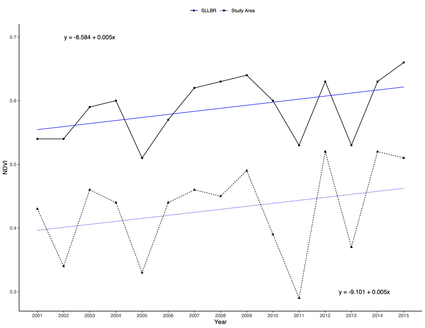
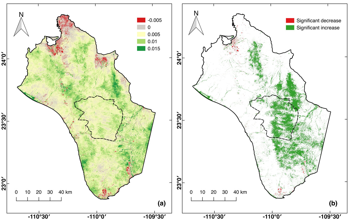
Figure 3 shows the general trend pattern of NDVI in the study area and the SLLBR polygon. As shown in this figure, from 2001 to 2015, an increasing pattern was observed in the NDVI values; the linear models suggested an increment of 0.005 per year in both the study area and the polygon. During the study period both areas had the lowest values in 2011 and the highest ones in 2014 and 2015. Spatial distribution of NDVI trend patterns are shown in figure 4a, which suggested that most of the study area had a positive and significant increase in the NDVI; however, areas close and within cities had a negative and significant decrease.

Table 1

Descriptive statistics (quartiles) of Normalised Difference Vegetation Index in the Cape Region, Baja California Sur, Mexico during the growing season (September – November) for the study period (2001-2015). In bold, the minimum and maximum NDVI values for each polygon.

Polygon	Veg. Type	Q0 (min)	Q1 (25%)	Q2 (50%)	Q3 (75%)	Q4 (max)	Mean	Std Dev
Study area	SRB	-0.452	0.283	0.359	0.442	0.687	0.361	0.112
	TDF	-0.165	0.464	0.543	0.603	0.739	0.542	0.098
	OW	-0.039	0.556	0.594	0.627	0.742	0.586	0.060
	OPW	0.289	0.570	0.591	0.611	0.706	0.589	0.035
	Urban area	-0.098	0.167	0.288	0.307	0.667	0.243	0.101
	Anthro. use	-0.177	0.292	0.359	0.434	0.693	0.364	0.118
SLLBR	SRB	0.074	0.460	0.536	0.569	0.680	0.505	0.101
	TDF	0.068	0.572	0.610	0.638	0.740	0.598	0.058
	OW	0.130	0.548	0.585	0.617	0.742	0.579	0.059
	OPW	0.289	0.570	0.591	0.611	0.706	0.589	0.035

Table 2

Classification of the coefficient of variation (CV) of Normalised Difference Vegetation Index (NDVI) and its percentage of surface area, in the Cape region, Baja California Sur, Mexico during the growing season (September – November) for the study period (2001-2015).

Polygon	Veg	Classification of variation
		Lower	Low	Moderate	High	Higher
Study area	SRB	1.72	11.09	20.46	34.16	32.56
	TDF	35.62	34.97	20.19	7.86	1.36
	OW	92.87	5.75	0.72	0.32	0.34
	OPW	99.74	0.22	0.03	0.01	0.00
	Urban areas	4.29	13.67	17.14	26.08	38.82
	Anthro. use	7.26	9.62	11.86	21.18	50.08
SLLBR	SRB	1.69	10.24	26.60	55.22	6.26
	TDF	67.14	23.50	6.91	1.88	0.57
	OW	92.93	5.98	0.62	0.25	0.23
	OPW	99.74	0.22	0.03	0.01	0.00

Trend values of NDVI by vegetation type are shown in Table 3. OW and OPW are the vegetation types that have increased in at least 40% of the study area. Although increasing patterns of SRB and TDF were lower than in other vegetation types, significant and positive values were greater than the significant and negative values.

Discussion

The Cape Region is characterised by the composition of its vegetation; it is located in an arid region with the tropical dry forest on the foothill of mountains and pine forest and oak-pine forest on the highlands (Fig.1). The results of this study showed that the highest NDVI values were located on highlands where radiation is intercepted by the canopy of evergreen oaks and pines of the woodland (León-de la Luz & Breceda, 2006); this result was consistent with that of the Moderate Resolution Imaging Spectrometer (MODIS) based-study carried out in Baja California Sur (Salinas-Zavala et al., 2017); the results of CV were also consistent where the variation on the Cape Region was less than 20% and within the reserve less than 10% in both studies (Salinas-Zavala et al., 2017).

The results indicated that the vegetation on the Cape Region has been increasing in recent years for all the different vegetation types; however, this result differs from a previously described trend in the same area, which showed negative NDVI trends, especially in the area of the pine-oak woodland within the SLLBR (Salinas-Zavala et al., 2017). This difference might be due to the spatial resolution, period of study and seasonal natural phenomena in relation to climate and plants. Salinas-Zavala et al. (2017) used data from MODIS with a 250 m spatial resolution, and they measured annual NDVI average for all months from 2001 to 2015. This result highlights the advantages of using Landsat products since they may have ideal sampling characteristics for monitoring diverse land cover types at a regional and historic level (Willis, 2015). The 30 m (900 m²) spatial resolution of Landsat sensor allows capturing spatial detail at a scale appropriate for monitoring vegetation structure and composition (Willis, 2015). MODIS has been widely used at regional scales; its pixel size of 250-500 m (62,500 m²-250,000 m²) makes it unsuitable for local scale studies but useful for long term and strategic regional planning (Nagendra et al., 2013).

The lowest NDVI and highest CV values were recorded close to and within the main cities in the study area where the populations and city sizes have increased considerably in the last 20 years, which suggested that the negative and significant trend of NDVI values were directly related with this growing population (INEGI, 2010, 2015). Most of the pixels with significant increases are primarily composed of tropical dry forest located in the easternmost area of study, which can be related with sea surface temperature, on both coasts, showing a range of differences from 5-10 ºC (Álvarez-Borrego, 2002). This situation affects, to a certain scale, regional environmental variables, such as the levels of air temperature, solar radiation and rainfall, aspects that determine predominance and even exclusion of some species on the eastern and western mountain slopes (León-de la Luz et al., 2012).

In the CR the dry season extends from November to late June (Díaz et al., 2001); thus, large number of plants experience challenging conditions and result in large variability of leaf health. Therefore, and to avoid this large variability, the growing season was selected to describe changes in the NDVI since this vegetation index has been used as a proxy for vegetation biomass productivity throughout the growing season (Gu & Wylie, 2015).

Interannual variations showed the maximum NDVI value (0.522) in 2014 and the minimum NDVI value (0.292) in 2011(Fig. 3). Near-shore tropical storm activity is a very important component of the annual rainfall in this region; for example, during Hurricane Juliet (27 September to 3 October 2001), San Bartolo station (∼23.75º N, 109.18º W) recorded 815 mm rainfall in 3 days when the annual mode was 400 mm and the mean was 319 mm (Díaz et al., 2008). The historical information about the cyclone season was analysed from 2001 to 2015 where 2001, 2003, 2006 and 2014 were the years most affected by hurricanes in the Cape Region, which coincides with some of the maximum peak NDVI values (SMN, 2018; Fig. 3).

Table 3

Trends and its percentage of surface area in the Cape Region, Baja California Sur, Mexico with significant pixel of Normalised Difference Vegetation Index by vegetation type during the growing season for the period 2001-2015.

Polygon	Veg	trend	% Area significance
			Decrease	Increase
Study area	SRB	0.005	0.19	6.16
	TDF	0.005	0.02	23.70
	OW	0.005*	0.01	52.88
	OPW	0.003	0.00	42.99
	UA	-0.001	10.53	6.64
	AU	0.004	1.29	16.85
SLLBR	SRB	0.004	0.27	88.73
	TDF	0.005	0.00	29.05
	OW	0.005*	0.00	53.82
	OPW	0.003	0.00	42.99

* corresponds to p < 0.05 (statistical significance of linear regression).

However, more detailed research is necessary to analyse the effectiveness of the reserve, and driving forces associated with vegetation variation should be explored, such as climate and topography. Whilst the area that is protected is an indicator of conservation inputs, this measure does not provide an assessment of conservation effectiveness in terms of habitat protection, preservation of biodiversity and/or prevention of habitat fragmentation (Nagendra, 2008; Nagendra et al., 2013; Nelson & Chomitz, 2011).

Acknowledgements

First author would like to thank Consejo Nacional de Ciencia y Tecnología for the scholarship provided. Also for the financial support (FONSEC-INEGI 278789 y CB 251919) and the Thematic Network RENANP-CONACyT. The authors thank Diana Fischer for editing and improving English quality of this manuscript.

References

Alvarez-Borrego, S. (2002). Physical oceanography. In Case T. J., Cody, M. L., & Ezcurra, E. (Eds.), A new island biogeography of the Sea of Cortés (pp. 41–59). New York, USA: Oxford University Press.

Arriaga, L., & Mercado, C. (2004). Seed bank dynamics and tree-fall gaps in a Northwestern Mexican Quercus-Pinus Forest. Journal of Vegetation Science, 15, 661–668. https://doi.org/10.1111/j.1654-1103.2004.tb02308.x

Arriaga, L., & Ortega-Rubio, A. (1988). La Sierra de la Laguna de Baja California Sur. México. Baja California Sur, Mexico: Centro Investigaciones Biologicas de Baja California Sur, A.C.

Bivand, R. (2018). RGdal: Bindings for the geospatial data abstraction library. R package 2.6–7. [Retrieved Nov. 2018]: https://cran.r-project.org/package=rgdal

Breceda, A., Sosa, J., Jiménez, C., & Ortega-Rubio, A. (2014). Conservación en la Reserva de la Biosfera Sierra la Laguna, Baja California Sur: logros y retos. Investigación y Ciencia de la Universidad Autónoma de Aguascalientes, 60, 78–84.

Conanp (Comisión Nacional de Áreas Naturales Protegidas). (2003). Programa de manejo Reserva de la Biosfera Sierra La Laguna. México D.F: Conanp.

Congedo, L. (2016). Semi-automatic classification plugin documentation. [Retrieved Nov. 2018] http://dx.doi.org/10.13140/RG.2.2.29474.02242/1

Corredor, X. (2018). CloudMasking Qgis plugin (version 18.2.7), SMByC-IDEAM and FAO. [Retrieved Nov. 2018]: https://smbyc.bitbucket.io/qgisplugins/cloudmasking

De Jong, R., de Bruin, S., de Wit, S., Schaepman, M. E., & Dent, D. L. (2011). Analysis of monotonic greening and browning trends from global NDVI time-series. Remote Sensing of Environment, 115, 692–702. https://doi.org/10.1016/j.rse.2010.10.011

Díaz, S. C., Salinas-Zavala, C. A., & Hernández-Vázquez, S. (2008). Variability of rainfall from tropical cyclones in north western Mexico and its relation to SOI and PDO. Atmosfera, 21, 213–223.

Díaz, S. C., Touchan, R., & Swetnam, T. W. (2001). A tree-ring reconstruction of past precipitation for Baja California Sur, Mexico. International Journal of Climatology, 21, 1007–1019. https://doi.org/10.1002/joc.664

Eckert, S., Hüsler, F., Linigier, H., & Hodel, E. (2015). Trend analysis of MODIS NDVI time series for detecting land degradation and regeneration in Mongolia. Journal of Arid Environments, 113, 16–28. https://doi.org/10.1016/j.jaridenv.2014.09.001

Franklin, A. B., Noon, B. R., & George, T. L. (2002). What is habitat fragmentation? Studies in Avian Biology, 25, 20–29.

García, E. (1973). Modificaciones al sistema de clasificación climática de Köppen. 2. Ed. Instituto de Geografía, Universidad Nacional Autónoma de México, Mexico.

Gillespie, T. W., Ostermann-Kelm, S., Dong, C., Willis, K. S., Okin, G. S., & Macdonald, G. M. (2018). Monitoring changes of NDVI in protected areas of southern California. Ecological Indicators, 88, 485–494. https://doi.org/10.1016/j.ecolind.2018.01.031

Gillespie, T. W, Willis, K., & Ostermann-Kelm, S. (2014). Spaceborne remote sensing of the world’s protected areas. Progress in Physical Geography, 39, 1–17. https://doi.org/10.1177/0309133314561648

Gu, X., & Wylie, B. K. (2015). Downsclaing 250-m MODIS growing season NDVI based on multiple-date Landsat images and data mining approaches. Remote Sensing, 7, 3489–3506. https://doi.org/10.3390/rs70403489

Hijmans, R. J. (2018). Raster: geographic data analysis and modeling. R package version 2.6–7. [Retrieved Nov. 2018]: https://cran.r-project.org/package=raster

Huang, C., Goward, S. N., Schleeweis, K., Thomas, N., Masek, J. F., & Zhu, Z. (2009). Dynamics of national forests assessed using the Landsat record: case studies in eastern United States. Remote Sensensing of Environment, 113, 1430–1442. https://doi.org/10.1016/j.rse.2008.06.016

INEGI (Instituto Nacional de Estadística y Geografía). (2010). Censos generales de población y vivienda. Tabulados básicos. Mexico: INEGI.

INEGI (Instituto Nacional de Estadística y Geografía). (2015). Encuesta intercensal. Tabulados básicos. Mexico: INEGI

INEGI (Instituto Nacional de Estadística y Geografía). (2016). Datos de uso del suelo y vegetación: escala 1:250,000: version 3. Mexico: INEGI

Jiang, W., Yuan, L., Wang, W., Cao, R., Zhang, Y., & Shen, W. (2015). Spatio-temporal analysis of vegetation variation in the Yellow River Basin. Ecological Indicators, 51, 117–126. https://doi.org/10.1016/j.ecolind.2014.07.031

León-de la Luz, J. L., & Breceda, A. (2006). Using endemic plant species to establish critical habitats in the Sierra de La Laguna Biosphere reserve, Baja California Sur, Mexico. Biodiversity & Conservation, 15, 1043–1055. https://doi.org/10.1007/s10531-004-3887-6

León-de la Luz, J. L., Domínguez-Cadena, R., & Medel-Narváez, A. (2012) Florística de la selva baja caducifolia de la península de Baja California, México. Botanical Sciences, 90, 143–162. https://doi.org/10.17129/botsci.480

León-de la Luz, J. L., Pérez-Navarro, J. J., & Breceda, A. (2000). A transitional xerophytic tropical plant community of the Cape Region, Baja California. Journal of Vegetation Science, 11, 555–564. https://doi.org/10.2307/3246585

Mallegowda, P., Rengaiang, G., Krishnan, J., & Niphadkar, M. (2015). Assessing habitat quality of forest-corridors through NDVI analysis in dry tropical forests of south India: implications for conservation. Remote Sensing, 7, 1619–1639. https://doi.org/10.3390/rs70201619

Milich, L., & Weiss, E. (2000). GAC NDVI inter annual coefficient of variation (CoV) images: ground truth sampling of the Sahel along north-south transects. International Journal of Remote Sensing, 21, 235–260. https://doi.org/10.1080/014311600210812

Nagendra, H. (2008). Do parks work? Impact of protected areas on land cover clearing. AMBIO:A Journal of the Human Environment, 37, 330–337. https://doi.org/10.1579/06-R-184.1

Nagendra, H., Lucas, R., Honrado, J. P., Jongman, R. H., Tarantino, C., Adamo, M., & Mairota, P. (2013). Remote sensing for conservation monitoring: assessing protected areas, habitat extent, habitat condition, species diversity, and threats. Ecological Indicators, 33, 45–59. https://doi.org/10.1016/j.ecolind.2012.09.014

Nelson, A., & Chomitz, K. M. (2011). Effectiveness of strict vs. multiple use protected areas in reducing tropical forest fires: a global analysis using matching methods. Plos One, 6, e22722. https://doi.org/10.1371/journal.pone.0022722

Padilla, G., Pedrin, S., & Díaz, E. (1988). Historia geológica y paleoecología, Arriaga, L., Ortega-Rubio, A. (Eds.), La Sierra de La Laguna en Baja California Sur. (pp. 27–36). Baja California Sur, Mexico: Centro de Investigaciones Biológicas de Baja California Sur, A. C.

Pang, G., Wang, X., & Yang, M. (2017). Using the NDVI to identify variations in, and responses of, vegetation to climate change on the Tibetan Plateau from 1982 to 2012. Quaternary International, 444, 87–96. https://doi.org/10.1016/j.quaint.2016.08.038

Peng, J., Liu, Z., Liu, Y., Wu, J., & Han, Y. (2012). Trend analysis of vegetation dynamics in Qinghai-Tibet Plateau using Hurst Exponent. Ecological Indicators, 14, 28–39. https://doi.org/10.1016/j.ecolind.2011.08.011

Prieto-Amparan, J., Villareal-Guerrero, F., Martínez-Salvador, M., Manjarrez-Domínguez, C., Santellano, E., & Pinedo-Álvarez, A. (2018). Atmospheric and radiometric correction algorithms for the multitemporal assessment of grasslands productivity. Remote Sensing, 10, 1–23. https://doi.org/10.3390/rs10020219

QGIS. Development Team. (2018). QGIS Geographic Information System. Open Source Geospatial Foundation. [Retrieved Jan. 2019]: http://qgis.org.

R Core Team. (2018). R: A language and environment for statistical computing. R Foundation for Statistical Computing, Vienna, Austria. [Retrieved Feb. 2019]: http://www.r-project.org/.

Rascón-Ayala, J. M., Alanís-Rodríguez, E., Mora-Olivio, A., Buenída-Rodríguez, E., Sánchez-Castillo, L., & Silva-García, J. E. (2018). Differences in vegetation structure and diversity of a forest in an altitudinal gradient of the Sierra La Laguna Biosphere Reserve, México. Botanical Sciences, 96, 598–608. https://doi.org/10.17129/botsci.1993

Rouse, J. W., Haas, R. H., Schell, J. A., & Deering, D. W. (1974). Monitoring vegetation systems in the great plains with ERTS. NASA Special Publication, 351, 309–318.

Salinas-Zavala, C. A., Martínez-Rincón, R. O., & Morales-Zarate, M. V. (2017). Trend in the Normalized Difference Vegetation Index (NDVI) in the Southern Part of Baja California Peninsula. Investigaciones Geográficas, 94, 82–90. http://dx.doi.org/10.14350/rig.57214

SMN (Sistema Meteorologico Nacional). (2018). Ciclones tropicales: información historica. [Retrieved Dec. 2018]: http://smn.cna.gob.mx/es/

Tucker, C. J., Newcomb, W. W., Los, S. O., & Prince, S. D. (2001). Mean and inter-year variation of growing-season normalized difference vegetation index for the Sahel 1981–1989. International Journal of Remote Sensing, 12, 1133–1135. https://doi.org/10.1080/01431169108929717

Willis, K. S. (2015). Remote sensing change detection for ecological monitoring in United States protected areas. Biological Conservation, 182, 233–242. https://doi.org/10.1016/j.biocon.2014.12.006